Models

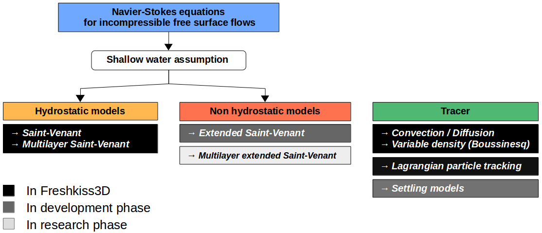
Due to computatonnal issues associated with the free surface Navier-Stokes equations, geophysical flows simulations are often carried out with reduced complexity models. With vertically averaged models such as the Saint-Venant system, the water height being an unknown of the system, there is no need to deal with moving meshes. Freshkiss3D’s numerical schemes are based on multilayer Saint-Venant systems with mass-exchanges (i.e. layer-averaged Euler or layer-averaged Navier-Stokes systems) of reduced complexity with respect to the Navier-Stokes equations but enriched with respect to the classic Shallow Water system. Layer-averaged models implemented in Freshkiss3D include topography, viscosity and friction source terms as well as variable density and tracer convection-diffusion.

In this section the Navier-Stokes with free surface system is presented in the introduction and then the focus is put on layer-averaged models implemented in Freshkiss3D. Given the complexity of the numerical methods involved, this documentation only scratches the surface of Freshkiss3D’s solver and it is highly recommended to refer to the References section.

I - System of equations for free surface flows

The fluid domain along \(z\) axis is delimited by free suface \(\eta(t,x,y)\) and topography \(z_b(x,y)\) and water depth is given by \(h(t,x,y)=\eta(t,x,y)-z_b(x,y)\).

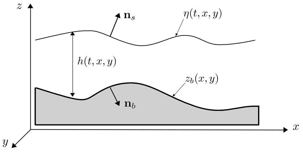
Fluid domain in (x,z) plane

I.1 - Incompressible Navier-Stokes equations with free surface

We consider the classical incompressible Navier-Stokes system:

\[\begin{split}\begin{eqnarray} \nabla. {\bf U}&=&0 \label{eq:nsi1}\\ \rho \left( \partial_t \bf U + \bf U. \nabla \bf U \right) &=& \nabla. \boldsymbol{\Sigma} +\rho {\bf g} \end{eqnarray}\end{split}\]

where the stress tensor \(\boldsymbol{\Sigma}\) is given by:

\[\boldsymbol{\Sigma} = -p \boldsymbol{I} + \mu [\nabla {\bf U}+(\nabla {\bf U})^T]\]

with \({\bf U}(t,x,y,z)=(u,v,w)^T\) the velocity, \(p\) the fluid pressure, \({\bf g}= ( 0,0,-g)^T\) the gravity forces, \(\mu\) the dynamic viscosity and \(\rho\) the density. The symbol \(\nabla\) denotes \(\nabla = \left(\partial_x, \partial_y, \partial_z \right)^{\top}\). Under the hydrostatic assumption, which consists in neglecting the vertical acceleration of the fluid, and under the Boussinesq assumption, which consists in neglecting the density variations in the acceleration terms, the system of equations becomes:

Important

(NS) The Navier-Stokes system with free surface:

\[\begin{split}\begin{align} \nabla. {\bf U} &= 0 \label{eq:incomp}\\ \partial_t {\bf u} + \nabla_{x,y}. ( {\bf u}\otimes {\bf u})+ \partial_z( {\bf u}w ) &= - \dfrac{1}{\rho_0} \nabla_{x,y} p + \nu \Delta {\bf u} \label{eq:mvthm}\\ \partial_z p &= - \rho g \label{eq:verticalihm} \end{align}\end{split}\]

with \({\bf u}(t,x,y,z)=(u,v)^T\) the horizontal velocity, \(\nu\) the kinematic viscosity defined by \(\mu/\rho_0\) and \(\nabla_{x,y}\) the horizontal projection of \(\nabla\).

I.2 - Tracer

The governing convection-diffusion equation for a tracer \(T\) inside the fluid domain is given by:

Important

(T) Tracer convection-diffusion equation:

\[\partial_t T + \nabla_{x,y}. ( {\bf u} T)+ \partial_z (wT) = \nu_T \Delta T\]

with \(\nu_T\) is defined by \(D_T/\rho_0\) with \(D_T\) the diffusion coefficient.

Note

In Freshkiss3D

• All default parameters are in the conf_dict.py file in the problem directory and could be changed (see details in Python API, problem)

• Tracers are optional and can be added to the simulation with the fk.Tracer class.

• By default the density \(\rho\) (see Navier-Stokes system) is set to \(\rho_0\) but can be set as a function of the tracer with the variable_density key of numerical_parameters in the fk.Problem class.

• The default density state laws included in Freshkiss3D can either take into account the effect of temperature, salinity and particle suspensions. See the parameters of the fk.Tracer class in the Python API.

I.3 - Boundary conditions and initial conditions

To complete the Navier-Stokes system with free surface boundary conditions and initial conditions have to be provided. Bottom and free surface kinematic and dynamic boundary conditions are defined in Freshkiss3D by:

\[\begin{split}\begin{cases} \partial_t \eta + {\bf U}_s . {\bf n}_s = 0 \\ {\bf U}_b . {\bf n}_b = 0 \end{cases}\end{split}\]

and:

\[\begin{split}\begin{cases} \boldsymbol{\Sigma}. \mathbf{n}_s = -p^{atm}.\mathbf{n}_s + \tau_w . \mathbf{t}_s \\ (\boldsymbol{\Sigma}. \mathbf{n}_b). \mathbf{t}_b = - \kappa_b(h,\mathbf{u}) \mathbf{u} .\mathbf{t}_b \end{cases}\end{split}\]

with \({\bf U}_s=U(t,x,y,z=\eta)\), \({\bf U}_b=U(t,x,y,z=Z)\), \({\bf n}_s\) and \({\bf n}_b\) the unit outwards normals at the free surface and bottom, \(p^{atm}\) the atmospheric pressure, \(\tau_w\) the wind shear stress at the free surface and \(\kappa_b(h,\mathbf{u})\) the friction coefficient.

Note

In Freshkiss3D (cf. Python API)

• \(\tau_w\) is optional and can be defined with the fk.WindEffect external effect class.

• \(\kappa_b(h,\mathbf{u})\) is optional and can be defined with the fk.Friction class.

On horizontal boundaries several types of boundary condition can be prescribed depending on the flow regime. The way of imposing these conditions depends on the layer-averaged model’s formulation and will not be detailed here. Additionally one has also to prescribe initial conditions to complete the model.

II - Layer-averaged models

Layer-averaged models are the core of Freshkiss3D and allow a 3D modelling of free surface flows. Depending on the initial hypotheses (i.e. user selected options) the models solved by Freshkiss3D behind the curtain can vary. In this section we briefly present some mathematical aspects of the vertical discretization as well as the different models obtained depending on various hypotheses. Some hints on how to select specific options are given with links to the Python API.

II.1 - Layerwise discretization

We consider a discretization of the fluid domain by layers where the layer \(\alpha\) contains the points of coordinates \((x,y,z)\) with \(z \in L_\alpha(t,x,y)= (z_{\alpha-1/2},z_{\alpha+1/2})\) and \(\{z_{\alpha+1/2}\}_{{\alpha} \in \{1,\dots,N \}}\) is defined for \(\alpha \in \{1,\dots,N \}\) by:

\[\begin{split}\left\{\begin{array}{l} z_{\alpha+1/2}(t,x,y) = z_b(x,y) + \sum_{j=1}^\alpha h_j(t,x,y) \\ h_\alpha(t,x,y) = z_{\alpha+1/2}(t,x,y) - z_{\alpha-1/2}(t,x,y)=l_\alpha h(t,x,y) \quad \text{with} \quad \sum_{\alpha=1}^N l_\alpha =1. \end{array}\right.\end{split}\]

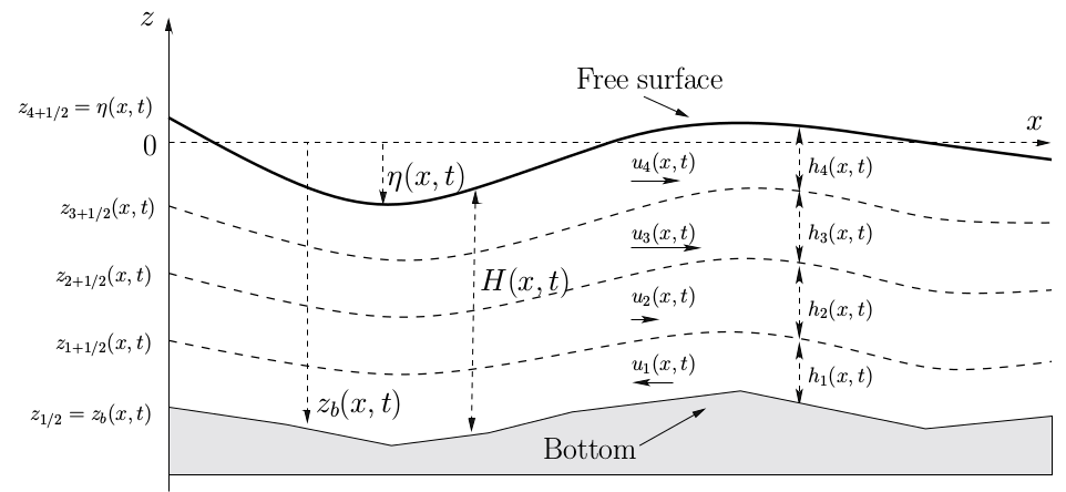
Fluid domain and layerwise discretization

Using the previous notations, let us consider the space \(\Bbb{P}_{0}\) of piecewise constant functions defined by

\[\Bbb{P}_{0} = \left\{ \mathbb{1}_{z \in L_\alpha(t,x,y)}(z),\quad \alpha\in\{1,\ldots,N\}\right\},\]

where \(\mathbb{1}_{z \in L_\alpha(t,x,y)}(z)\) is the characteristic function of the layer \(L_\alpha(t,x,y)\). Using this formalism, the projection of \(u\), \(v\), \(w\) and \(T\) on \(\Bbb{P}_{0}\) is a piecewise constant function defined by:

\[X(t,x,y,\{z_\alpha\}) = \sum_{\alpha=1}^N \mathbb{1}_{[z_{\alpha-1/2},z_{\alpha+1/2}]}(z)X_\alpha(t,x,y),\]

Note that the free surface changing over time, the \(\Bbb{P}_{0}\) space as well as the piecewise constant function projections are time dependent.

II.2 - The layer-averaged Euler system

Let us first neglect the viscosity and assume that the density is constant (i.e. \(\rho =\rho_0\)). Using the space \(\Bbb{P}_0\) and the above decomposition, the Galerkin approximation of the incompressible and hydrostatic Euler equations leads to the system:

Important

(LE.1) The layer-averaged Euler system:

for \(\alpha \in \{1,\dots,N \}\):

\[\begin{split}\begin{eqnarray} &&\sum_{\alpha=1}^N \frac{\partial h_\alpha }{\partial t } + \sum_{\alpha=1}^N \nabla_{x,y} . (h_\alpha {\bf u} _\alpha) =0\\ &&\frac{\partial h_{\alpha}{\bf u}_{\alpha}}{\partial t} + \nabla_{x,y} .\left(h_{\alpha} {\bf u}_{\alpha} \otimes {\bf u}_{\alpha} \right) + \nabla_{x,y} \bigl(\frac{g}{2} h h_{\alpha}\bigr) = -gh_\alpha \nabla_{x,y} z_b \nonumber\\ && \qquad + {\bf u}_{\alpha+1/2} G_{\alpha+1/2} - {\bf u}_{\alpha-1/2} G_{\alpha-1/2} \end{eqnarray}\end{split}\]

The quantity \(G_{\alpha+1/2}\) (resp. \(G_{\alpha-1/2}\)) corresponds to the mass exchange accross the interface \(z_{\alpha+1/2}\) (resp. \(z_{\alpha-1/2}\)) and \(G_{\alpha+1/2}\) is defined by:

\[\begin{split}\begin{eqnarray} %G_{1/2} & = & 0\nonumber\\ G_{\alpha+1/2} %& = &\frac{\partial z_{\alpha+1/2}}{\partial t} + u_{\alpha+1/2} \frac{\partial z_{\alpha+1/2}}{\partial x} + v_{\alpha+1/2} \frac{\partial z_{\alpha+1/2}}{\partial y} - w(x,y,z_{\alpha+1/2},t)\nonumber\\ & = & \sum_{j=1}^\alpha \left(\frac{\partial h_j}{\partial t } + \nabla_{x,y} . (h_j {\bf u}_j) \right) = -\sum_{j=1}^N \Bigl(\sum_{p=1}^\alpha l_p - \mathbb{1}_{j\leq \alpha}\Bigr)\nabla_{x,y} . (h_j {\bf u}_j), \end{eqnarray}\end{split}\]

for \(\alpha=1,\ldots,N\). The velocities at the interfaces \({\bf u}_{\alpha+1/2}\) are defined by:

\[\begin{split}{\bf u}_{\alpha+1/2} = \left\{\begin{array}{ll} {\bf u}_\alpha & if \;G_{\alpha+1/2} \leq 0\\ {\bf u}_{\alpha+1} & if \;G_{\alpha+1/2} > 0 \end{array}\right.\end{split}\]

For smooth solutions, the system (LE.1) satisfies an energy balance (see References for complete proof). Note that the vertical velocity is not an unknown of the system but can be computed considering the divergence free condition and we obtain the following piecewise approximation of the vertical velocity:

\[\begin{split}w_{\alpha} = k_{\alpha} - z_{\alpha} \nabla_{x,y}.{\bf u}_{\alpha} \quad \text{with:} \quad \begin{cases} k_1 = \nabla_{x,y} . (z_b{\bf u}_{1})\\ k_{\alpha+1} = k_{\alpha} + \nabla_{x,y} . (z_{\alpha+1/2} ({\bf u}_{\alpha+1} - {\bf u}_{\alpha} )) \end{cases}\end{split}\]

Also note that when the number of layers is equal to one, the classical Saint-Venant system with topography is obtained:

Important

(SV) The Saint-Venant system:

\[\begin{split}\begin{eqnarray} &&\frac{\partial h}{\partial t} + \nabla_{x,y} . (h {\bf u})= 0 \\ &&\frac{\partial h {\bf u}}{\partial t} + \nabla_{x,y} . \left(h {\bf u} \otimes {\bf u} + g \frac{h^2}{2} \right) = -gh \nabla_{x,y} z_b \end{eqnarray}\end{split}\]

Note

In Freshkiss3D (cf. Python API)

• The layer-averaged Euler system is solved by default when no other option is selected

• Layers are defined with the fk.Layer class which is initialized with a user defined number of layers:NL.

Applying the same decomposition to the tracer equation gives:

Important

(LT) The layer-averaged tracer equation:

for \(\alpha \in \{1,\dots,N \}\):

\[\begin{eqnarray} \frac{\partial h_\alpha T_\alpha }{\partial t } + \nabla_{x,y} . (h_\alpha {\bf u}_\alpha T_\alpha) = T_{\alpha+1/2} G_{\alpha+1/2} - T_{\alpha-1/2} G_{\alpha-1/2} \end{eqnarray}\]

where \(G_{\alpha+1/2}\) and \(G_{\alpha-1/2}\) are defined as in (II.2).

II.3 - The layer-averaged Euler system with variable density

As mentioned before, the variable density model relies on the Boussinesq assumption, which means that the variable density only appears in the gravity term. When the density is not constant, integrating the vertical pressure gradient leads to a slighly different model as one cannot assume \(p=\rho_0 g (\eta-z)\) anymore. Now \(p = g \int_{z}^{\eta} \rho dz\). Again, using piecewise approximation one can write the pressure as:

\[p(x,y,z,t) = g \left( \rho_{\alpha} (z_{\alpha+1/2}-z) + \sum_{j=\alpha+1}^{N} \rho_j h_j \right)\]

The Galerkin approximation of the incompressible and hydrostatic Euler equations with variable density leads to the system:

Important

(LE.2) The layer-averaged Euler system with variable density:

for \(\alpha \in \{1,\dots,N \}\):

\[\begin{split}\begin{eqnarray} &&\sum_{\alpha=1}^N \frac{\partial h_\alpha }{\partial t } + \sum_{\alpha=1}^N \nabla_{x,y} . (h_\alpha {\bf u} _\alpha)=0\\ &&\frac{\partial h_{\alpha}{\bf u}_{\alpha}}{\partial t} + \nabla_{x,y} .\left(h_{\alpha} {\bf u}_{\alpha} \otimes {\bf u}_{\alpha} \right) + \nabla_{x,y} (h_{\alpha} p_{\alpha}) = {\bf u}_{\alpha+1/2} G_{\alpha+1/2} - {\bf u}_{\alpha-1/2} G_{\alpha-1/2}\\ && \qquad + p_{\alpha+1/2} \nabla_{x,y} z_{\alpha+1/2} - p_{\alpha-1/2} \nabla_{x,y} z_{\alpha-1/2}\\ &&\frac{\partial h_\alpha T_\alpha }{\partial t } + \nabla_{x,y} . (h_\alpha {\bf u}_\alpha T_\alpha) = T_{\alpha+1/2} G_{\alpha+1/2} - T_{\alpha-1/2} G_{\alpha-1/2} \end{eqnarray}\end{split}\]

where \(G_{\alpha+1/2}\) (resp. \(G_{\alpha-1/2}\)), \(z_{\alpha+1/2}\) (resp. \(z_{\alpha-1/2}\)), \({\bf u}_{\alpha+1/2}\) (resp. \({\bf u}_{\alpha-1/2}\)) are defined as in (LE.1), \(\rho_{\alpha}=f(T_{\alpha})\) with \(f\) a state law and \(p_{\alpha}\), \(p_{\alpha+1/2}\) are defined by:

\[\begin{split}\begin{cases} p_{\alpha} = \frac{1}{h_{\alpha}} \int_{z_{\alpha-1/2}}^{z_{\alpha+1/2}} p(x,y,z,t)dz = g \left( \frac{\rho_{\alpha} h_{\alpha}}{2} + \sum_{j=\alpha +1}^{N} \rho_j h_j \right)\\ p_{\alpha+1/2} = p(x,y,z_{\alpha+1/2},t) = g \sum_{j=\alpha +1}^{N} \rho_j h_j \end{cases}\end{split}\]

Note

In Freshkiss3D (cf. Python API)

• As mentionned before, variable density model can be activated by setting the variable_density key of numerical_parameters to True.

• The ipres key of numerical_parameters allows the user to select the pressure term formulation of (LE.2) instead of (LE.1) even if \(\rho\) is set to constant, in which case \(\rho_{\alpha}\) is replaced in all equations by \(\rho_0\) and the tracer is optional. Note that when boussinesq is prescribed, ipres is automatically set to True and tracer is mandatory.

II.4 - The layer-averaged Navier-Stokes system

Let us now apply the same process to the complete Navier-Stokes with free surface system (NS), so that viscosity and friction terms are added to the system. Note that it can be done with or without variable density but only the constant \(\rho\) case is presented for sake of simplicity. From now on we denote \(\bf \Sigma\) as the x,y projection of the 3D stress tensor.

Important

(LNS.1) The layer-averaged Navier-Stokes system:

for \(\alpha \in \{1,\dots,N \}\):

\[\begin{split}\begin{eqnarray} &&\sum_{\alpha=1}^N \frac{\partial h_\alpha }{\partial t } + \sum_{\alpha=1}^N \nabla_{x,y} . (h_\alpha {\bf u} _\alpha) =0\\ &&\frac{\partial h_{\alpha}{\bf u}_{\alpha}}{\partial t} + \nabla_{x,y} .\left(h_{\alpha} {\bf u}_{\alpha} \otimes {\bf u}_{\alpha} \right) + \nabla_{x,y} \bigl(\frac{g}{2} h h_{\alpha}\bigr) = -gh_\alpha \nabla_{x,y} z_b \nonumber\\ && \qquad + {\bf u}_{\alpha+1/2} G_{\alpha+1/2} - {\bf u}_{\alpha-1/2} G_{\alpha-1/2} + \nabla_{x,y} . \bigl( h_\alpha {\bf \Sigma}_\alpha \bigr) \nonumber\\ && \qquad - {\bf \Sigma}_{\alpha+1/2} \nabla_{x,y} z_{\alpha+1/2} + {\bf \Sigma}_{\alpha-1/2} \nabla_{x,y} z_{\alpha-1/2} \nonumber\\ && \qquad +2\mu_{\alpha+1/2} \frac{{\bf u}_{{\alpha}+1}-{\bf u}_{\alpha}}{h_{{\alpha}+1}+h_{\alpha}} - 2\mu_{\alpha-1/2} \frac{{\bf u}_{\alpha}-{\bf u}_{{\alpha}-1}}{h_{\alpha}+h_{{\alpha}-1}} -\kappa_{\alpha}{\bf u}_{\alpha} \end{eqnarray}\end{split}\]

where \(G_{\alpha+1/2}\) (resp. \(G_{\alpha-1/2}\)), \(z_{\alpha+1/2}\) (resp. \(z_{\alpha-1/2}\)), \({\bf u}_{\alpha+1/2}\) (resp. \({\bf u}_{\alpha-1/2}\)) are defined as in (LE.1) and the stress tensor terms are defined by:

\[\begin{split}\begin{eqnarray} {\bf \Sigma}_{\alpha+1/2} & = & \begin{pmatrix} \Sigma_{xx,\alpha+1/2} & \Sigma_{xy,\alpha+1/2}\\ \Sigma_{yx,\alpha+1/2} & \Sigma_{yy,\alpha+1/2} \end{pmatrix}\\ \Sigma_{xx,\alpha+1/2} & = & \frac{\mu_{\alpha+1/2}}{h_{\alpha+1}+h_\alpha}\bigl( h_{\alpha}\frac{\partial u_{\alpha}}{\partial x} + h_{\alpha+1}\frac{\partial u_{\alpha+1}}{\partial x} \bigr) - 2 \mu_{\alpha+1/2}\frac{\partial z_{\alpha+1/2}}{\partial x} \frac{u_{\alpha+1} - u_\alpha}{h_{\alpha+1} + h_\alpha}\\ \Sigma_{xy,\alpha+1/2} & = & \frac{\mu_{\alpha+1/2}}{h_{\alpha+1}+h_\alpha}\bigl( h_{\alpha}\frac{\partial u_{\alpha}}{\partial y} + h_{\alpha+1}\frac{\partial u_{\alpha+1}}{\partial y} \bigr) - 2 \mu_{\alpha+1/2}\frac{\partial z_{\alpha+1/2}}{\partial y} \frac{u_{\alpha+1} - u_\alpha}{h_{\alpha+1} + h_\alpha}\\ {\bf \Sigma}_{\alpha} & = & \begin{pmatrix} \Sigma_{xx,\alpha} & \Sigma_{xy,\alpha}\\ \Sigma_{yx,\alpha} & \Sigma_{yy,\alpha} \end{pmatrix} = \frac{{\bf \Sigma}_{\alpha+1/2}+ {\bf \Sigma}_{\alpha-1/2}}{2} \end{eqnarray}\end{split}\]

with the friction and viscosity coefficients given by:

\[\begin{split}\begin{equation} \kappa_{\alpha}= \left\{ \begin{array}{l} \kappa \quad {\rm if} \quad \alpha =1\\ 0 \quad {\rm if} \quad\alpha \ne 1 \end{array} \right. \quad \mu_{\alpha+1/2}= \left\{ \begin{array}{l} 0 \quad {\rm if} \quad \alpha =0\\ \mu \quad {\rm if} \quad\alpha \in \{1,...,N-1 \} \\ 0\quad {\rm if} \quad\alpha=N \end{array}\right. \end{equation}\end{split}\]

with \(\kappa\) the Navier friction coefficient and \(\mu\) the dynamic viscosity

For smooth solutions, the system (LNS.1) satisfies an energy balance (see References for complete proof). The viscous terms in the layer-averaged Navier-Stokes sytem are difficult to discretise so only a simplified version of this model is implemented into Freshkiss3D (see References section for details).

Also note that when the number of layers is equal to one, the viscous Saint-Venant system with topography is obtained. In this case, the friction coefficient can be chosen amongst a wide variety of empirical laws. Note that only the constant \(\kappa\) (Navier friction law) is relevant when \(NL>1\).

Important

(VSV) The viscous Saint-Venant system:

\[\begin{split}\begin{eqnarray} &&\frac{\partial h}{\partial t} + \nabla_{x,y} . (h {\bf u})= 0 \\ &&\frac{\partial h {\bf u}}{\partial t} + \nabla_{x,y} . \left(h {\bf u} \otimes {\bf u} + g \frac{h^2}{2} \right) = -gh \nabla_{x,y} z_b - \kappa(h,{\bf u}).{\bf u} + \nabla_{x,y} . (h {\bf \Sigma}) \end{eqnarray}\end{split}\]

with \(\kappa(h,{\bf u})\):

• Navier: \(\kappa(h,{\bf u}) = \kappa\)

• Chézy: \(\kappa(h,{\bf u}) = \frac{g |{\bf u}|}{C_h^2}\)

• Strikler: \(\kappa(h,{\bf u}) = \frac{g}{S_t^2} \left( \frac{|{\bf u}|}{h^{1/3}} \right)\)

• Manning: \(\kappa(h,{\bf u}) = g M_a^2 \left( \frac{|{\bf u}|}{h^{1/3}} \right)\)

Note

In Freshkiss3D (cf. Python API)

• Viscosity can be toggled by setting the horizontal_viscosity and vertical_viscosity keys of the physical_parameters dictionary.

• Friction can be toggled by setting the friction_coeff and friction_law keys of the physical_parameters dictionary. Note that friction can also be added to the layer-averaged Euler system when viscosity is set to zero.

• friction_law is set to 'Navier' by default

• When NL=1 user can choose between several friction_law including

Important

The Saint-Venant system with coriolis force:

\[\begin{split}\frac{\partial h }{\partial t } + \nabla_{x,y}\cdot (h {\bf u} ) =0, \\ \frac{\partial (h{\bf u})}{\partial t} + \nabla_{x,y} \cdot\left( h {\bf u} \otimes {\bf u} \right) + \nabla_{x,y} \bigl(\frac{g}{2} h^2\bigr) = -gh \nabla_{x,y} z_b -\Omega h{\bf u}^\perp.\end{split}\]

Note

In Freshkiss3D (cf. Python API)

• Coriolis force might be applied by setting the coriolis_effect keys of the physical_parameters dictionary. The user can choose to pass \(\Omega(x, y)\) to Coriolis_coeff attribut of fk.primitive by an array or a constant or a function.

III - Numerical scheme

The layer-averaged Navier-Stokes system has the form:

\[\partial_t U + \nabla_{x,y} . F(U) = S_b(U) + S_e(U) + S_{v,f}(U)\]

where the state vector is defined by:

\[U=\left(h, q_{x,1}, \ldots, q_{x,N}, q_{y,1}, \ldots, q_{y,N}\right)^T\]

with \(q_{x,\alpha}=h_\alpha u_{\alpha}\), \(q_{y,\alpha}=h_\alpha v_{\alpha}\). \(F(U)\) stands for the fluxes of the conservative part, and \(S_b(U)\), \(S_e(U)\) and \(S_{v,f}(U)\) are the source terms, representing respectively the topography effects, the momentum exchanges and the viscous and friction effects.

III.1 - Time discretization

Let us denote discrete times by \(t^n\) and \(t^{n+1}=t^n+\Delta t^n\). For the time discretisation of the layer-averaged Navier-Stokes system a time splitting technique is adopted to treat the conservative part, the vertical exchanges and the viscous part successively:

\[\begin{split}\begin{cases} U^* = U^n - \Delta t^n \left( \nabla_{x,y} . F(U^n) - S_b(U^n) \right) \\ \tilde{U} = U^* + \Delta t^n S_e(\tilde{U}, G(U^{n}))\\ U^{n+1} = \tilde{U} + \Delta t^n S_{v,f}(U^{n+1}, \tilde{U}) \end{cases}\end{split}\]

The conservative part is fully explicit and includes the topography source term which is treated with a well-balanced hydrostatic reconstruction scheme. The vertical exchanges terms are semi-implicit, \(G\) being computed with \(U^{n}\). The viscous and friction effects are semi-implicit as well, the horizontal viscosity being fully explicit and the vertical viscosity and friction (treated at the same time) fully implicit. The coriolis force is an semi-implicit.

Noting \(U^{n+1} = U^n + \Delta t^n f(U^n)\) the fully explicit first order scheme, the second order scheme extension implemented in Freshkiss3D, based on a modified version of the Heun scheme, is:

\[\begin{split}\begin{cases} U^{(1)} = U^n + \Delta t_1^n f(U^n) \\ U^{(2)} = U^{(1)} + \Delta t_2^{n} f(U^{(1)}) \\ U^{n+1} = (1 - \gamma) U^n + \gamma U^{(2)} \end{cases}\end{split}\]

with:

\[\Delta t^n = \frac{2\Delta t_1^n\Delta t _2^n}{\Delta t_1^n + \Delta t_2^n}, \quad \gamma = \frac{(\Delta t^n)^2}{2 \Delta t_1^n \Delta t_2^n}\]

Since \(\gamma \geq 0\), \(U^{n+1}\) is a convex combination of \(U^n\) and \(U^{(2)}\) so the scheme preserves the positivity. For the previous relations \(\Delta t_1^{n}\) and \(\Delta t_2^{n}\) respectively satisfy the CFL conditions associated with \(U^n\) and \(U^{(1)}\).

Note

In Freshkiss3D (cf. Python API)

• Time discretization parameters are passed to fk.Problem class via the fk.Simutime class.

• By default time step \(\Delta t^n\) is computed with a CFL condition to ensure stability. The default CFL number is set to 0.9 but can be changed with the parameter cfl_adjuster key of the numerical_parameters dictionary. Although it is not recommended, the user can force a constant time step by passing constant_dt to fk.Simutime.

• In fk.Simutime you can set the second_order to True to select second order time scheme.

• By default semi-implicit methods are used for \(S_e\) and \(S_{v,f}\) but the user can switch back to fully explicit methods by setting implicit_exchanges and implicit_vertical_viscosity parameters to False in the fk.Problem class.

III.2 - Space discretization

Let \(\Omega\) denote the computational domain with boundary \(\Gamma\), which we assume is polygonal. Let \(T_h\) be a triangulation of \(\Omega\) for which the vertices are denoted by \(P_i\) with \(S_i\) the set of interior nodes and \(G_i\) the set of boundary nodes. For the space discretization of the system, we use an hybrid method. A finite volume technique is used for the conservative part and exchange terms and a \(\Bbb{P}_1\) finite element approach on \(T_h\) for the viscous part.

We recall now the general formalism of finite volumes on unstructured meshes. The dual cells \(C_i\) are obtained by joining the centers of mass of the triangles surrounding each vertex \(P_i\). We use the following notations:

• \(K_i\), set of subscripts of nodes \(P_j\) surrounding \(P_i\),

• \(|C_i|\), area of \(C_i\),

• \(\Gamma_{ij}\), boundary edge between the cells \(C_i\) and \(C_j\),

• \(L_{ij}\), length of \(\Gamma_{ij}\),

• \({\bf n}_{ij}\), unit normal to \(\Gamma_{ij}\), outward to \(C_i\) (\({\bf n}_{ji}= -{\bf n}_{ij}\)).

If \(P_i\) is a node belonging to the boundary \(\Gamma\), we join the centers of mass of the triangles adjacent to the boundary to the middle of the edge belonging to \(\Gamma\) and we denote

• \(\Gamma_i\), the two edges of \(C_i\) belonging to \(\Gamma\),

• \(L_i\), length of \(\Gamma_i\) (for sake of simplicity we assume in the following that \(L_i = 0\) if \(P_i\) does not belong to \(\Gamma\)),

• \({\bf n}_i\), the unit outward normal defined by averaging the two adjacent normals.

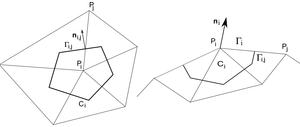
Dual cell \(C_i\) and bondary cell.

Note

In Freshkiss3D (cf. Python API)

• The triangular mesh is passed to the fk.Problem class via the fk.TriangularMesh class.

• The fk.TriangularMesh class can be defined from a file with fk.TriangularMesh.from_msh_file('file.msh')

• Freshkiss3D mesh IO supports 3 different mesh formats for your mesh file: FreeFem++ .msh, Medit .mesh and Gmsh .msh (format msh2).

• See the Meshes section of the Gallery of examples to learn how to manipulate meshes with Freshkiss3D

We define the piecewise constant functions \(U^n(x,y)\) on cells \(C_i\) corresponding to time \(t^n\) and \(z_b(x,y)\) as:

\[U^n(x,y)= U^n_i,\quad z_b(x,y)= z_{b,i},\quad\mbox{ for } (x,y)\in C_i\]

with \(U^n_i = (h^n_i,q^n_{x,1,i},\ldots,q^n_{x,N,i},q^n_{y,1,i},\ldots,q^n_{y,N,i})^T\) i.e. \(U^n_i \approx \frac{1}{|C_i|}\int_{C_i} U(t^n,x,y)dxdy\), \(z_{b,i} \approx \frac{1}{|C_i|}\int_{C_i} z_b(x,y)dxdy\). We will also use the notation \(U^n_{\alpha,i} \approx \frac{1}{|C_i|}\int_{C_i}U_\alpha(t^n,x,y)dxdy\). A finite volume scheme for solving the conservative part is:

\[U^{*}_i=U^n_i- \sum_{j\in K_i} \sigma_{i,j}{\cal F}_{i,j} - \sigma_i {\cal F}_{e,i}\]

\[\sum_{j\in K_i} L_{i,j} {\cal F}_{i,j} \approx \int_{C_i} \nabla_{x,y} . F(U^n) dx dy,\]

with \(\sigma_{i,j} = \frac{\Delta t^nL_{i,j}}{|C_i|},\quad \sigma_{i} = \frac{\Delta t^nL_{i}}{|C_i|}\). Here we consider first-order explicit schemes where:

\[{\cal F}_{i,j} = F(U^n_i,U^n_j,z^n_{b,i}-z^n_{b,j},{\bf n}_{i,j}) \quad \text{and} \quad {\cal F}_{e,i} = F(U^n_i,U^n_{e,i},{\bf n}_{i})\]

The term \(\cal{F}_{i,j}\) denotes an interpolation of the normal component of the flux \(F(U^n). {\bf n}_{i,j}\) along the edge \(C_{i,j}\). The functions \(F(U^n_i,U^n_j,z^n_{b,i} - z^n_{b,j},{\bf n}_{i,j})\in {\cal R}^{2N+1}\) are the numerical fluxes which are computed using a kinetic interpretation of the system (see References). The source terms discretization (vertical exchanges, viscosity,…) as well as the second order scheme have been omitted but are detailed in reference papers (see References).

Note

In Freshkiss3D (cf. Python API)

• In fk.Problem you can either set second_order parameter or second_order key of numerical_parameters dictionary to True in order to select the second order space scheme.

III.3 - Initial conditions

Initial conditions are needed to define initial state vector:

\[U^0=\left(h^0, q^0_{x,1}, \ldots, q^0_{x,N}, q^0_{y,1}, \ldots, q^0_{y,N}\right)^T\]

as well as initial values for topography: \(z^0_b\). By default all variables are set to zero in Freshkiss3D if no initial values are provided.

Note

In Freshkiss3D (cf. Python API):

• The topography is initialized when calling the fk.Layer class presented above.

• The state vector containing U, V, H, HL, QX, and QY variables is defined with the fk.Primitive class. Initialization takes place when declaring this class for the first time using init parameters, the types of which can be constant float, vector or function.

• As mentioned before the tracer T is defined and initialized in fk.Tracer class.

III.4 - Boundary conditions

In order to complete the numerical scheme, one has to provide boundary conditions, i.e. to define the fluxes \({\cal F}_{e,i} = F(U^n_i,U^n_{e,i},{\bf n}_{i})\).

Note

In Freshkiss3D (cf. Python API), boundary conditions are selected with the following class:

• fk.FluvialFlowRate: fluvial regime fluid boundary condition with given flow rate.

• fk.FluvialHeight: fluvial regime fluid boundary condition with given water depth.

• fk.TorrentialOut: torrential regime fluid boundary condition with free outlet.

• fk.Slide: solid wall boundary with slip condition \({\bf u} \cdot {\bf n} = 0\).

• fk.DampingOut: damp waves with coefficient \(\theta\) ; \(\partial_t \bf X = -\theta ({\bf X} - {\bf X}^0)\).

• Time varying boundary conditions can be passed to fk.FluvialFlowRate and fk.FluvialHeight using fk.TimeDependentFlowRate and fk.TimeDependentHeight.