Construct a Mesh from a .msh file

Mesh is constructed from a .msh and plotted.

import matplotlib.pyplot as plt
import numpy as np
import freshkiss3d as fk
import freshkiss3d.extra.plots as fk_plt

Read a Mesh

There is two ways to visualize a mesh from a file. You can either build a TriangularMesh or directly use the read_msh function.

TG, vertex_labels, boundary_labels = fk.read_msh('inputs/tiny.msh')

Warning

The read_msh function is compatible with .msh, .msh (GMSH) and .mesh (MEDIT) formats ONLY. Note that the .msh used in freshkiss3d isn’t the same as gmsh .msh format.

Construct a TriangularMesh

triangular_mesh = fk.TriangularMesh.from_msh_file('inputs/tiny.msh')

TG = triangular_mesh.triangulation
vertex_labels = triangular_mesh.vertex_labels
boundary_edges = triangular_mesh.boundary_edges

Note

When you build a TriangularMesh, the read_msh function is called in the background

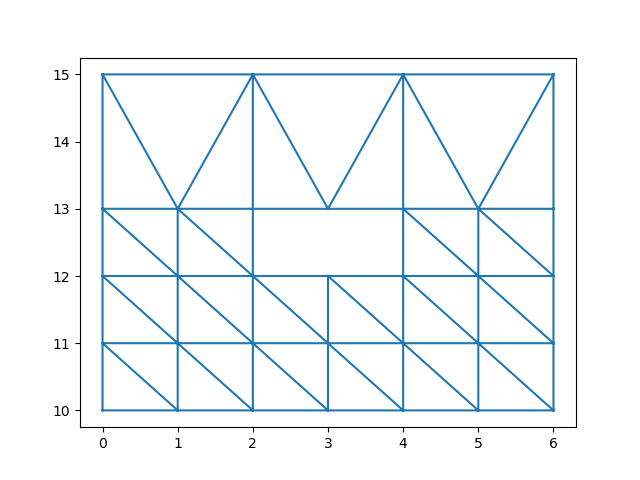
Basic plot

To visualize the mesh with triplot you need to recover nodes coordonates (x,y) and triangles (trivtx)

x = np.asarray(TG.x)
y = np.asarray(TG.y)
trivtx = np.asarray(TG.trivtx)

plt.triplot(x, y, trivtx)
plt.show()

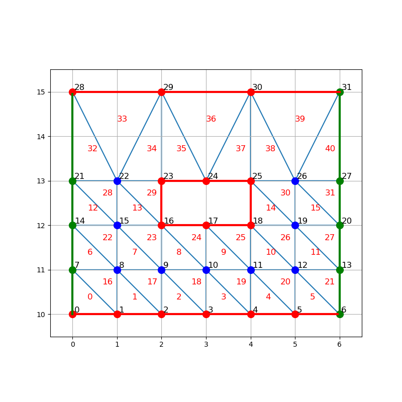
Fancy plot

Basic plot isn’t really helpfull when you need specific information about your mesh, for example node or boundary labels. So here is shown how to add life to your mesh plots:

colors = {0:'blue', 1:'red', 2:'green'}
plt.figure(figsize=(8, 8))

 # Plot triangles.
plt.triplot(x, y, trivtx)
xtri = np.average(x[trivtx], axis=1)
ytri = np.average(y[trivtx], axis=1)
fk_plt.put_text_index(xtri, ytri, color='red')

# Plot points.
for a, b, label in zip(x, y, vertex_labels):
    plt.plot(a, b, marker='o', color=colors[label], markersize=10)
fk_plt.put_text_index(x, y, offset=(0.04, 0.04))

# Plot edges.
for B in range(boundary_edges.size):
    i0 = boundary_edges.vertices[B, 0]
    i1 = boundary_edges.vertices[B, 1]
    x0, y0 = x[i0], y[i0]
    x1, y1 = x[i1], y[i1]
    plt.plot([x0, x1], [y0, y1], color=colors[boundary_edges.label[B]], linewidth=3.)

plt.grid()
plt.axis('scaled')
plt.xlim(-0.5, 6.5)
plt.ylim(9.5, 15.5)
plt.show()