Note
Click here to download the full example code
Bump
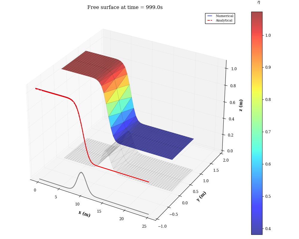
In this example the classic test of the bump for the Saint-Venant system is illustrated. Comparison between 2D numerical solution and 1D analytical solution is carried out for three flow regimes.
Note
1D analytical solutions are given in: https://hal.archives-ouvertes.fr/hal-00628246/document at section 3.1, paragraph “Bumps”.
import os, sys
import argparse
import numpy as np
import matplotlib.pylab as plt
import freshkiss3d as fk
import freshkiss3d.extra.plots as fk_plt

parser = argparse.ArgumentParser()
parser.add_argument('--nographics', action='store_true')
args = parser.parse_args()

#sphinx_gallery_thumbnail_number = 2
Flow regimes:
From the properties of the single layer St Venant system (strict hyperbolicity) we can deduce a classification of flows based on a criticality condition. Let’s first define the Froude number:
The flow can be either subcritical or supercritical (Fr<1 and Fr>1 respectively). For a given discharge another usefull quantity is the critical height defined by :
The flow is subcritical and supercritical for h>h_c and h<h_c respectively
In this example, several cases are considered depending on boundary conditions:
Subcritical flow
Transcritical flow without shock : the flow becomes torrential at the top of the bump.
Transcritical flow with shock : the flow becomes torrential at the top of the bump and fluvial again after the shock
FLOW = 'trans'

if FLOW == 'sub':
    FREE_SURFACE_0 = 0.7
    Q_IN = 0.2
if FLOW == 'trans':
    FREE_SURFACE_0 = 0.7
    Q_IN = 1.5
if FLOW == 'trans_shock':
    FREE_SURFACE_0 = 0.33
    Q_IN = 0.18

H_OUT = FREE_SURFACE_0
FINAL_TIME = 1000.
Time loop:
simutime = fk.SimuTime(final_time=FINAL_TIME, time_iteration_max=100000,
                       second_order=True)

# Plot figure scheduler:
WHEN = [FINAL_TIME-1.]
create_figure_scheduler = fk.schedules(times=WHEN)
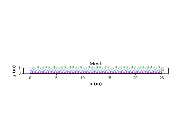
Mesh:
\[L = 25 m, l = 1 m\]
dir_path = os.path.abspath(os.path.dirname(sys.argv[0]))
triangular_mesh = fk.TriangularMesh.from_msh_file(dir_path+'/inputs/bump.mesh')

if not args.nographics:
  fk_plt.plot_mesh(triangular_mesh)
1D Steady state analytic solutions:
1D steady state analytic solution is defined in a Bump class. Computation of the solution depends on intial state, boundary conditions and flow type. The topography is defined as a function of x:
X_B = 10.
def topo(x):
    if 8.< x <12.:
        topo = 0.2 - 0.05*(x-X_B)**2
    else:
        topo = 0.0
    return topo

def topo_gaussian(x):
    topo = 0.25*np.exp(-0.5*(x-X_B)**2)
    return topo

bump_analytic = fk.Bump(triangular_mesh,
                        case=FLOW,
                        q_in=Q_IN,
                        h_out=H_OUT,
                        x_b = X_B,
                        free_surface_init=FREE_SURFACE_0,
                        topo = topo_gaussian,
                        scheduler=fk.schedules(times=WHEN))
bump_analytic(0.)
In the ‘subcritical’ case, analytical solution is given by the resolution of:
\[h(x)^3 + \left( z(x) - \dfrac{q_0^2}{2g h(L)^2} - h(L) \right) h(x)^2 + \dfrac{q_0^2}{2g} = 0 \quad \forall x \in [0,L]\]
In the ‘transcritical’ case without shock, analytical solution is given by the resolution of:
\[h(x)^3 + \left( z(x) - \dfrac{q_0^2}{2g h_c^2} - h_c - z_M \right) h(x)^2 + \dfrac{q_0^2}{2g} = 0 \quad \forall x \in [0,L]\]\[\text{where } z_M = \max_{x \in [0,L]}z\]
In the ‘transcritical’ case with shock, analytical solution is given by the resolution of:
\[\begin{split}\begin{cases} h(x)^3 + \left( z(x) - \dfrac{q_0^2}{2g h_c^2} - h_c - z_M \right) h(x)^2 + \dfrac{q_0^2}{2g} = 0 \quad & \text{for } x < x_{shock} \\ h(x)^3 + \left( z(x) - \dfrac{q_0^2}{2g h(L)^2} - h(L) \right) h(x)^2 + \dfrac{q_0^2}{2g} = 0 \quad &\text{for } x < x_{shock} \\ q_0^2 \left( \dfrac{1}{h(x_{shock}^-)} - \dfrac{1}{h(x_{shock}^+)} \right) + \dfrac{g}{2} \left( h(x_{shock}^-)^2 -h(x_{shock}^+)^2 \right) = 0 \end{cases}\end{split}\]
Warning
Analytic solution is available in Bump for 1D steady state, single layer St Venant only
Layers:
Number of layers is set to one for comparison with analytical solutions.
Note
Topography defined in fk.Bump is shared with fk.Layer
NL=1
layer = fk.Layer(NL, triangular_mesh, topography=bump_analytic.topography)
Primitives:
primitives = fk.Primitive(triangular_mesh, layer,
                          free_surface=FREE_SURFACE_0,
                          QXinit=Q_IN,
                          QYinit=0.)
Boundary conditions:
fluvial_flowrates = [fk.FluvialFlowRate(ref=1,
                                        flowrate=Q_IN,
                                        x_flux_direction=1.0,
                                        y_flux_direction=0.0)]

fluvial_heights = [fk.FluvialHeight(ref=2, height=H_OUT)]
torrential_outs = [fk.TorrentialOut(ref=2)]

slides = [fk.Slide(ref=3), fk.Slide(ref=4)]
Problem definition:
if FLOW == 'sub' or 'trans_shock':
    problem = fk.Problem(simutime, triangular_mesh,
                         layer, primitives,
                         fluvial_flowrates=fluvial_flowrates,
                         fluvial_heights=fluvial_heights,
                         slides=slides,
                         numerical_parameters={'space_second_order':True},
                         analytic_sol=bump_analytic,
                         custom_funct={'plot':fk_plt.plot_freesurface_3d_analytic},
                         custom_funct_scheduler=create_figure_scheduler)

elif FLOW == 'trans':
    problem = fk.Problem(simutime, triangular_mesh,
                         layer, primitives,
                         fluvial_flowrates=fluvial_flowrates,
                         torrential_outs=torrential_outs,
                         slides=slides,
                         numerical_parameters={'space_second_order':True},
                         analytic_sol=bump_analytic,
                         custom_funct={'plot':fk_plt.plot_freesurface_3d_analytic},
                         custom_funct_scheduler=create_figure_scheduler)
===================================================================
|                          INITIALIZATION                         |
===================================================================
Problem size: Nodes=149, Layers=1, Triangles=196,
Iter =        0 ; Dt = 0.0000s ; Time =     0.00s ; ETA =     0.00s
Problem solving:
problem.solve()

if not args.nographics:
  plt.show()
===================================================================
|                            TIME LOOP                            |
===================================================================
Iter =     1662 ; Dt = 0.0117s ; Time =    20.41s ; ETA =    68.69s
Iter =     3450 ; Dt = 0.0114s ; Time =    40.82s ; ETA =    66.48s
Iter =     5247 ; Dt = 0.0114s ; Time =    61.24s ; ETA =    57.03s
Iter =     7043 ; Dt = 0.0114s ; Time =    81.64s ; ETA =    57.39s
Iter =     8839 ; Dt = 0.0114s ; Time =   102.04s ; ETA =    63.13s
Iter =    10635 ; Dt = 0.0114s ; Time =   122.45s ; ETA =    60.62s
Iter =    12432 ; Dt = 0.0114s ; Time =   142.87s ; ETA =    51.10s
Iter =    14228 ; Dt = 0.0114s ; Time =   163.27s ; ETA =    52.48s
Iter =    16024 ; Dt = 0.0114s ; Time =   183.67s ; ETA =    50.54s
Iter =    17821 ; Dt = 0.0114s ; Time =   204.09s ; ETA =    54.68s
Iter =    19617 ; Dt = 0.0114s ; Time =   224.49s ; ETA =    46.41s
Iter =    21413 ; Dt = 0.0114s ; Time =   244.90s ; ETA =    46.89s
Iter =    23210 ; Dt = 0.0114s ; Time =   265.32s ; ETA =    51.20s
Iter =    25006 ; Dt = 0.0114s ; Time =   285.72s ; ETA =    44.14s
Iter =    26802 ; Dt = 0.0114s ; Time =   306.12s ; ETA =    43.48s
Iter =    28599 ; Dt = 0.0114s ; Time =   326.54s ; ETA =    42.57s
Iter =    30395 ; Dt = 0.0114s ; Time =   346.95s ; ETA =    47.46s
Iter =    32191 ; Dt = 0.0114s ; Time =   367.35s ; ETA =    45.17s
Iter =    33988 ; Dt = 0.0114s ; Time =   387.77s ; ETA =    37.19s
Iter =    35784 ; Dt = 0.0114s ; Time =   408.17s ; ETA =    35.41s
Iter =    37580 ; Dt = 0.0114s ; Time =   428.58s ; ETA =    34.84s
Iter =    39376 ; Dt = 0.0114s ; Time =   448.98s ; ETA =    34.04s
Iter =    41173 ; Dt = 0.0114s ; Time =   469.40s ; ETA =    32.10s
Iter =    42969 ; Dt = 0.0114s ; Time =   489.80s ; ETA =    30.94s
Iter =    44765 ; Dt = 0.0114s ; Time =   510.20s ; ETA =    30.10s
Iter =    46562 ; Dt = 0.0114s ; Time =   530.62s ; ETA =    28.51s
Iter =    48358 ; Dt = 0.0114s ; Time =   551.03s ; ETA =    27.48s
Iter =    50154 ; Dt = 0.0114s ; Time =   571.43s ; ETA =    26.85s
Iter =    51951 ; Dt = 0.0114s ; Time =   591.85s ; ETA =    24.87s
Iter =    53747 ; Dt = 0.0114s ; Time =   612.25s ; ETA =    23.65s
Iter =    55543 ; Dt = 0.0114s ; Time =   632.66s ; ETA =    22.36s
Iter =    57340 ; Dt = 0.0114s ; Time =   653.07s ; ETA =    20.81s
Iter =    59136 ; Dt = 0.0114s ; Time =   673.48s ; ETA =    20.07s
Iter =    60932 ; Dt = 0.0114s ; Time =   693.88s ; ETA =    24.71s
Iter =    62729 ; Dt = 0.0114s ; Time =   714.30s ; ETA =    20.74s
Iter =    64525 ; Dt = 0.0114s ; Time =   734.70s ; ETA =    16.10s
Iter =    66321 ; Dt = 0.0114s ; Time =   755.11s ; ETA =    15.22s
Iter =    68117 ; Dt = 0.0114s ; Time =   775.51s ; ETA =    14.00s
Iter =    69914 ; Dt = 0.0114s ; Time =   795.93s ; ETA =    12.76s
Iter =    71710 ; Dt = 0.0114s ; Time =   816.33s ; ETA =    11.39s
Iter =    73506 ; Dt = 0.0114s ; Time =   836.74s ; ETA =     9.83s
Iter =    75303 ; Dt = 0.0114s ; Time =   857.15s ; ETA =     8.41s
Iter =    77099 ; Dt = 0.0114s ; Time =   877.56s ; ETA =     7.47s
Iter =    78895 ; Dt = 0.0114s ; Time =   897.96s ; ETA =     6.12s
Iter =    80692 ; Dt = 0.0114s ; Time =   918.38s ; ETA =     4.91s
Iter =    82488 ; Dt = 0.0114s ; Time =   938.78s ; ETA =     3.81s
Iter =    84284 ; Dt = 0.0114s ; Time =   959.19s ; ETA =     2.46s
Iter =    86081 ; Dt = 0.0114s ; Time =   979.60s ; ETA =     1.22s
===================================================================
|                      L2 errors at time 999 s:
|                           H : 0.004279
|                          QX : 0.004768
|                          QY : 0.000000
===================================================================
Iter =    87877 ; Dt = 0.0049s ; Time =  1000.00s ; ETA =     0.00s
===================================================================
|                               END                               |
===================================================================
Problem.solve() completed in 63.85642147064209s (wall time)
Total running time of the script: ( 1 minutes 4.276 seconds)