Note
Click here to download the full example code
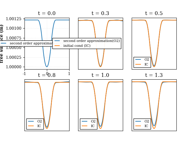
Stationnary vortex
In this example, we test the conservation of the geostrophic equilibrium by conserving a stationnary vortex. The test case is already discribed in [10] and [11] (see References).
import os, sys
from os import listdir
import argparse
import matplotlib.pylab as plt
import freshkiss3d as fk
import freshkiss3d.extra.plots as fk_plt
import numpy as np
import matplotlib.tri as mtri
from scipy.interpolate import griddata
from matplotlib import colors
import matplotlib.ticker as mtick
import h5py
import math

#sphinx_gallery_thumbnail_number = 2

parser = argparse.ArgumentParser()
parser.add_argument('--nographics', action='store_true')
args = parser.parse_args()

fk_plt.set_rcParams()


def plot_free_surface_slice(triangular_mesh, H, topography, fig,
    nb_l, nb_c, plt_num,
    time, Eta0_slice=None, label=True):
    # Plt options:
    n = 100
    TG = triangular_mesh.triangulation
    x_slice = np.linspace(min(TG.x), max(TG.x), n)
    ym_slice = np.full(n, (max(TG.y) + min(TG.y)) / 2.0)

    NC = triangular_mesh.NV
    Eta = np.empty(NC, dtype='d')
    for C in range(NC):
        Eta[C] = H[C] + topography[C]

    Eta_slice = griddata((TG.x, TG.y), Eta, (x_slice, ym_slice), method = 'cubic')


    ax = fig.add_subplot(nb_l, nb_c, plt_num)
    ax.xaxis.set_major_formatter(mtick.FormatStrFormatter('%d'))
    if label:
        ax.plot(x_slice, Eta_slice, label='second order approximation(O2)')
    else:
        ax.plot(x_slice, Eta_slice, label='O2')

    if Eta0_slice is not None:
        if label:
            ax.plot(x_slice, Eta0_slice, label='initial cond (IC)')
        else:
            ax.plot(x_slice, Eta0_slice, label='IC')
        ax.get_xaxis().set_visible(False)
        ax.get_yaxis().set_visible(False)

    ax.set_xlim([min(x_slice), max(x_slice)])
    ax.set_ylabel("free surface (m)")
    ax.set_title("t = {:.1f}".format(time))
    ax.legend(loc='best')

    return Eta_slice


dir_path = os.path.abspath(os.path.dirname(sys.argv[0]))
Analytic solution:
The hydrostatic Euler with Coriolis and constant density is given by
First, we consider the reference case given in polar coordinates. In this case, the problem is initialized with the velocity \({\bf{u}}^0\) and the water height \(h^0\),
with:
In cartesian coordinates, this gives :
with:
def hVortex(r, h0):
    if 0. <= r and r <= 0.2:
        return h0 + (omega + 5 * eps) * (r ** 2) * 2.5 * eps / g
    elif 0.2 < r and r <= 0.4:
        return hVortex(0.2, h0) + eps * \
        omega / g * (2 * r - 2.5 * (r ** 2) - 0.3) \
        + (eps ** 2) / g * (4 * np.log(5 * r) - 20 * r + 12.5 * r ** 2 + 3.5)
    elif 0.4 < r:
        return hVortex(0.4, h0)


def uVortex(r): # u_theta
    return eps * (5 * r * (r <= 0.2) + (2 - 5 * r) * (0.2 < r and r <= 0.4))
Parameters:
We assume that \(\rho = \rho_0 = 1\). In the [11], authors of choose \(\alpha = 5 \varepsilon\), where \(\varepsilon\) controls the depth of the vortex, and \(R = \frac{1}{5}\).
# Non-linear vortex:
omega = 1. # angular velocity

#Let us consider two cases:
#
# * In the first case we use a semi-implicite in time method
# * In the second case we use the apparent topography method, the method is only implemented for the order 1.
#


case = 1
if case == 1:
    NUM_PARAMS={'space_second_order':True}
    PHY_PARAMS={'coriolis_effect':True, 'apparent_topo':False}

if case == 2:
    NUM_PARAMS={'space_second_order':False}
    PHY_PARAMS={'coriolis_effect':True, 'apparent_topo':True}

g = 9.81
h0 = 1. # initial water height
eps = 0.05 # controls the depth of the vortex
# the smaller it is, the closer you are to the linear
Time loop:
FINAL_TIME = 1.5
simutime = fk.SimuTime(final_time=FINAL_TIME, time_iteration_max=1000000,
                       second_order=True)
restart_times = [0., 0.25, 0.5, 0.75, 1., 1.25]
restart_scheduler = fk.schedules(times=restart_times)
Mesh:
Also we consider a square domain \([-1, 1] \times [-1, 1]\), the average edge length of the mesh equals to 0.04.
os.system('gmsh -2 -format msh2 inputs/tiny_square.geo -o inputs/tiny_square.msh')

triangular_mesh = \
    fk.TriangularMesh.from_msh_file(
    dir_path + '/inputs/tiny_square.msh')
hm = 0.04
Layers:
NL = 1
layer = fk.Layer(NL, triangular_mesh, topography=0.)
LAYER_IDX = int(NL/2)
Primitives:
NC = triangular_mesh.NV
x = triangular_mesh.vertices.x
y = triangular_mesh.vertices.y

h_init = np.empty(NC, dtype='d')
hu_init = np.empty((NC, NL), dtype='d')
hv_init = np.empty((NC, NL), dtype='d')

for C in range(NC):
    rt = np.sqrt(x[C] ** 2 + y[C] ** 2)
    al = np.arctan2(y[C], x[C])
    h_init[C] = hVortex(rt, h0)
    for L in range(NL):  # Correct for only one layer
        hu_init[C,L] = h_init[C] * (-np.sin(al) * uVortex(rt))
        hv_init[C,L] = h_init[C] * (np.cos(al) * uVortex(rt))

primitives = fk.Primitive(triangular_mesh, layer,
                          height=h_init,
                          QXinit=hu_init,
                          QYinit=hv_init,
                          Coriolis_coeff=omega)
Boundary conditions:
slides = [fk.Slide(ref=r) for r in [1, 2, 3, 4]]
Writter:
vtk_writer = fk.VTKWriter(triangular_mesh,
                          scheduler=fk.schedules(count=10), scale_h=10.)

h5_writer = fk.H5Writer(scheduler=restart_scheduler, \
    output_dir='outputs/hydrodynamic_h5_vortex')
Problem definition:
problem = fk.Problem(simutime, triangular_mesh,
                     layer, primitives,
                     slides=slides,
                     numerical_parameters=NUM_PARAMS,
                     physical_parameters=PHY_PARAMS,
                     vtk_writer=vtk_writer,
                     h5_writer=h5_writer,
                     )
===================================================================
|                          INITIALIZATION                         |
===================================================================
Problem size: Nodes=3014, Layers=1, Triangles=5826,
Iter =        0 ; Dt = 0.0000s ; Time =     0.00s ; ETA =     0.00s
Problem solving:
problem.solve()
===================================================================
|                            TIME LOOP                            |
===================================================================
Iter =       26 ; Dt = 0.0012s ; Time =     0.03s ; ETA =    12.92s
Iter =       51 ; Dt = 0.0012s ; Time =     0.06s ; ETA =    12.46s
Iter =       76 ; Dt = 0.0012s ; Time =     0.09s ; ETA =    12.30s
Iter =      101 ; Dt = 0.0012s ; Time =     0.12s ; ETA =    11.90s
Iter =      126 ; Dt = 0.0012s ; Time =     0.15s ; ETA =    11.33s
Iter =      151 ; Dt = 0.0012s ; Time =     0.18s ; ETA =    10.75s
Iter =      176 ; Dt = 0.0012s ; Time =     0.22s ; ETA =    10.64s
Iter =      201 ; Dt = 0.0012s ; Time =     0.25s ; ETA =    10.42s
Iter =      226 ; Dt = 0.0012s ; Time =     0.28s ; ETA =    10.09s
Iter =      251 ; Dt = 0.0012s ; Time =     0.31s ; ETA =     9.86s
Iter =      276 ; Dt = 0.0012s ; Time =     0.34s ; ETA =     9.43s
Iter =      301 ; Dt = 0.0012s ; Time =     0.37s ; ETA =     9.33s
Iter =      326 ; Dt = 0.0012s ; Time =     0.40s ; ETA =     9.09s
Iter =      351 ; Dt = 0.0012s ; Time =     0.43s ; ETA =     8.75s
Iter =      376 ; Dt = 0.0012s ; Time =     0.46s ; ETA =     8.45s
Iter =      401 ; Dt = 0.0012s ; Time =     0.49s ; ETA =     8.22s
Iter =      426 ; Dt = 0.0012s ; Time =     0.52s ; ETA =     7.98s
Iter =      451 ; Dt = 0.0012s ; Time =     0.55s ; ETA =     7.96s
Iter =      476 ; Dt = 0.0012s ; Time =     0.58s ; ETA =     7.66s
Iter =      501 ; Dt = 0.0012s ; Time =     0.61s ; ETA =     7.45s
Iter =      526 ; Dt = 0.0012s ; Time =     0.64s ; ETA =     7.18s
Iter =      551 ; Dt = 0.0012s ; Time =     0.67s ; ETA =     6.85s
Iter =      576 ; Dt = 0.0012s ; Time =     0.71s ; ETA =     6.60s
Iter =      601 ; Dt = 0.0012s ; Time =     0.74s ; ETA =     6.32s
Iter =      626 ; Dt = 0.0012s ; Time =     0.77s ; ETA =     6.13s
Iter =      651 ; Dt = 0.0012s ; Time =     0.80s ; ETA =     5.87s
Iter =      676 ; Dt = 0.0012s ; Time =     0.83s ; ETA =     5.56s
Iter =      701 ; Dt = 0.0012s ; Time =     0.86s ; ETA =     5.36s
Iter =      726 ; Dt = 0.0012s ; Time =     0.89s ; ETA =     5.13s
Iter =      751 ; Dt = 0.0012s ; Time =     0.92s ; ETA =     4.77s
Iter =      776 ; Dt = 0.0012s ; Time =     0.95s ; ETA =     4.51s
Iter =      801 ; Dt = 0.0012s ; Time =     0.98s ; ETA =     4.32s
Iter =      826 ; Dt = 0.0012s ; Time =     1.01s ; ETA =     3.95s
Iter =      851 ; Dt = 0.0012s ; Time =     1.04s ; ETA =     3.79s
Iter =      876 ; Dt = 0.0012s ; Time =     1.07s ; ETA =     3.50s
Iter =      901 ; Dt = 0.0012s ; Time =     1.10s ; ETA =     3.26s
Iter =      926 ; Dt = 0.0012s ; Time =     1.13s ; ETA =     3.04s
Iter =      951 ; Dt = 0.0012s ; Time =     1.16s ; ETA =     2.78s
Iter =      976 ; Dt = 0.0012s ; Time =     1.19s ; ETA =     2.50s
Iter =     1001 ; Dt = 0.0012s ; Time =     1.23s ; ETA =     2.27s
Iter =     1026 ; Dt = 0.0012s ; Time =     1.26s ; ETA =     2.03s
Iter =     1051 ; Dt = 0.0012s ; Time =     1.29s ; ETA =     1.76s
Iter =     1076 ; Dt = 0.0012s ; Time =     1.32s ; ETA =     1.51s
Iter =     1101 ; Dt = 0.0012s ; Time =     1.35s ; ETA =     1.26s
Iter =     1126 ; Dt = 0.0012s ; Time =     1.38s ; ETA =     0.99s
Iter =     1151 ; Dt = 0.0012s ; Time =     1.41s ; ETA =     0.75s
Iter =     1176 ; Dt = 0.0012s ; Time =     1.44s ; ETA =     0.51s
Iter =     1201 ; Dt = 0.0012s ; Time =     1.47s ; ETA =     0.25s
Iter =     1226 ; Dt = 0.0002s ; Time =     1.50s ; ETA =     0.00s
===================================================================
|                               END                               |
===================================================================
Problem.solve() completed in 14.015119075775146s (wall time)
Plot the data saved
TIMES = []
H_t = []


filenames = [f for f in listdir('./outputs/hydrodynamic_h5_vortex')]
filenames = ['./outputs/hydrodynamic_h5_vortex/' + f for f in filenames]
order = [int(f[-4]) for f in filenames]
filenames = [f for _,f in sorted(zip(order, filenames))]

for filename in filenames:
    h5_reader = fk.H5Reader(filename = filename)
    x,_y, time, time_it_, H, U, V, W, HL, QX, QY, Rho, \
        topography , Hn, Un, Vn, \
        HLn, QXn, QYn, T, HT, Tn, HTn, positions, velocities = \
        h5_reader.read_solution()

    TIMES.append(time)
    H_t.append(H)

if not args.nographics:
    nb_l = 2
    nb_c = 3
    pos = 1
    fig = plt.figure(1)

    Eta0_slice = plot_free_surface_slice(\
            triangular_mesh, H_t[0], topography, fig,
            nb_l, nb_c, pos, TIMES[0])

    N_TIMES = len(TIMES)
    for i in range(1, N_TIMES):
        pos += 1
        label = True
        if i != 1:
            label = False
        plot_free_surface_slice(\
            triangular_mesh, H_t[i], topography, fig,
            nb_l, nb_c, pos, TIMES[i], Eta0_slice=Eta0_slice, label=label
        )

plt.show()

os.system('rm inputs/tiny_square.msh')
0
Total running time of the script: ( 0 minutes 15.232 seconds)