Analytical solutions¶

Example of analytical solution computing.

import os
import numpy as np
import matplotlib.pyplot as plt
from matplotlib import cm
import matplotlib.tri as mtri
import freshkiss3d as fk
import freshkiss3d.extra.plots as fk_plt

Plotting functions:¶

Visualization are scaled by a factor 2 in the z-direction.

scale = 2.
def create_figure(time):
    plt.rcParams["figure.figsize"] = [10, 8]
    fig = plt.figure()
    ax = fig.add_subplot(111, projection='3d')
    H = np.asarray(thacker2d_analytic.H)
    z = np.asarray(thacker2d_analytic.topography)
    elevation = np.asarray(thacker2d_analytic.elevation)
    NT = triangular_mesh.NT
    triang = mtri.Triangulation(x, y, trivtx)
    triang2 = mtri.Triangulation(TG.x, TG.y, TG.trivtx)
    #set-up masked triangles:
    isbad = np.ndarray( (NT), dtype=bool)
    for T in range(NT):
        eps = 1.e-5
        V0 = TG.trivtx[T,0]
        V1 = TG.trivtx[T,1]
        V2 = TG.trivtx[T,2]
        isbad_0 = np.greater(eps, H[V0])
        isbad_1 = np.greater(eps, H[V1])
        isbad_2 = np.greater(eps, H[V2])
        isbad[T] = isbad_0 or isbad_1 or isbad_2
    triang.set_mask(isbad)
    ax.plot_trisurf(triang2, scale*z, lw=0.01, edgecolor="w", color='grey', alpha=0.2)
    csetb = ax.tricontour(triang2, scale*z, 1, zdir='x', offset=4, color='grey')
    csetb = ax.tricontour(triang2, scale*z, 1, zdir='y', offset=0, color='grey')
    ax.plot_trisurf(triang, scale*elevation, lw=0.0, edgecolor="w", cmap=cm.jet,alpha=0.9)
    cset = ax.tricontour(triang, scale*elevation, 1, zdir='x', offset=4, cmap=cm.coolwarm)
    cset = ax.tricontour(triang, scale*elevation, 1, zdir='y', offset=0, cmap=cm.coolwarm)
    ax.set_title("Free surface at time={}".format(time))

Mesh:¶

os.system('gmsh -2 -format msh2 ../simulations/inputs/thacker2d_huge.geo -o inputs/thacker2d.msh')
TG, vertex_labels, boundary_labels = fk.read_msh('inputs/thacker2d.msh')
os.system('rm inputs/thacker2d.msh')

x = np.asarray(TG.x)
y = np.asarray(TG.y)
trivtx = np.asarray(TG.trivtx)

x *= 0.4
y *= 0.4

triangular_mesh = fk.TriangularMesh(TG, vertex_labels, boundary_labels)

Define analytic solution:¶

First a object Thacker2D containning the thacker 2d analytic solution needs to be declared:

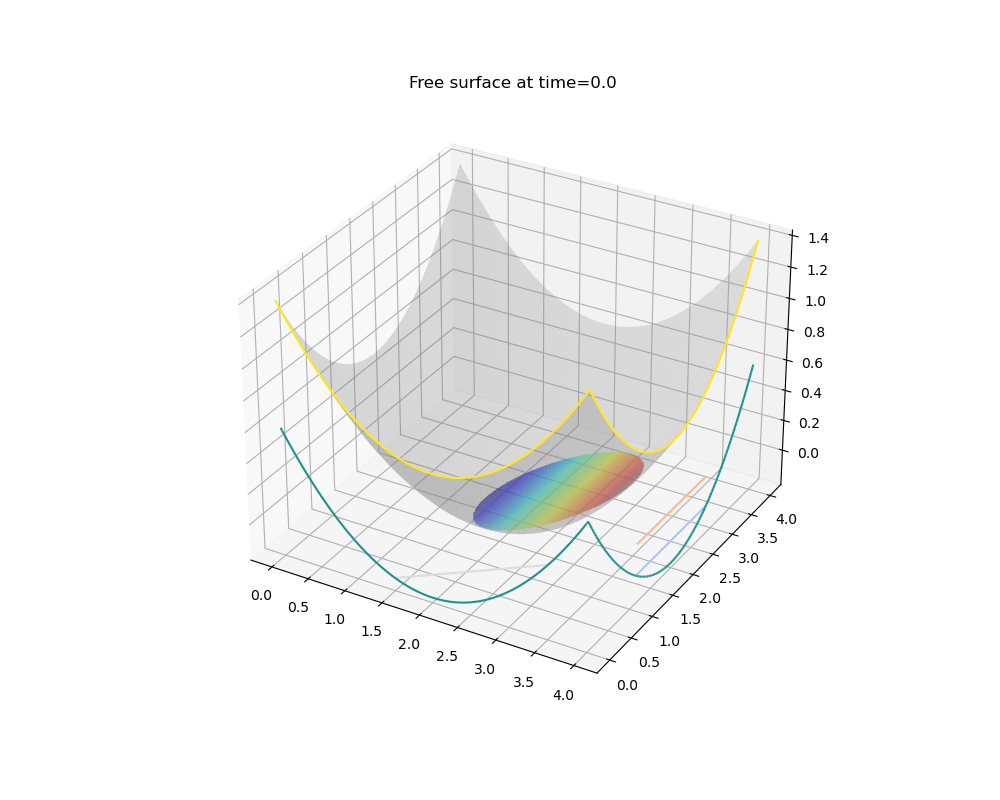
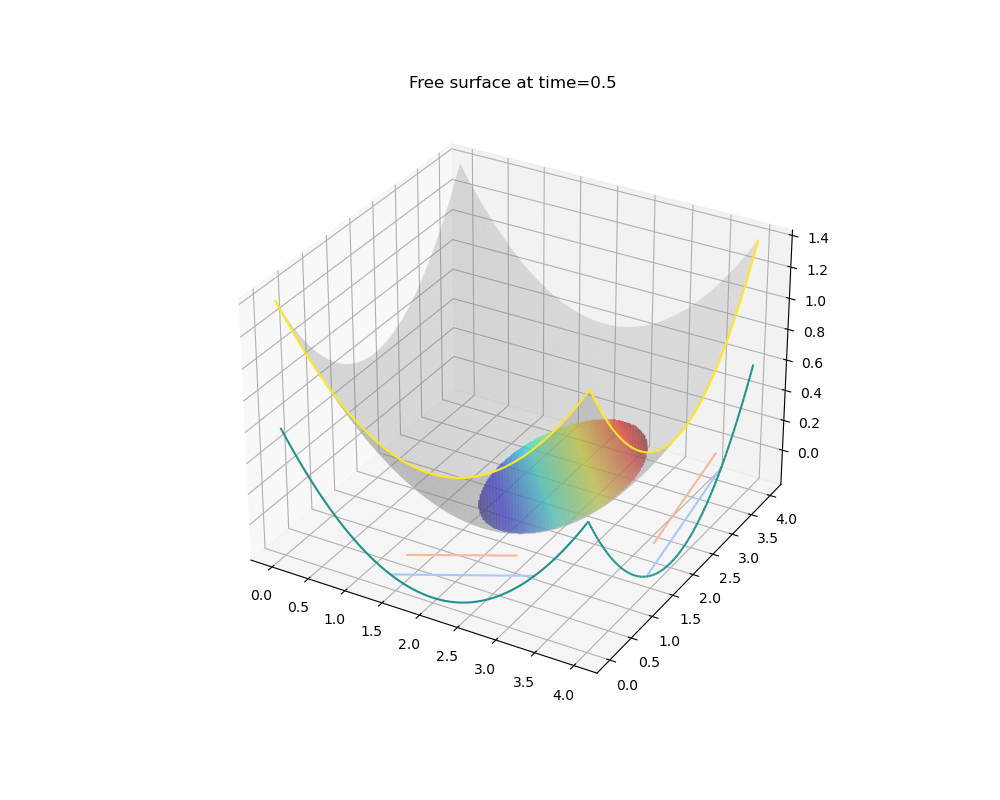
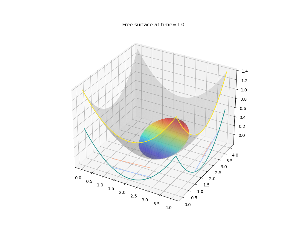
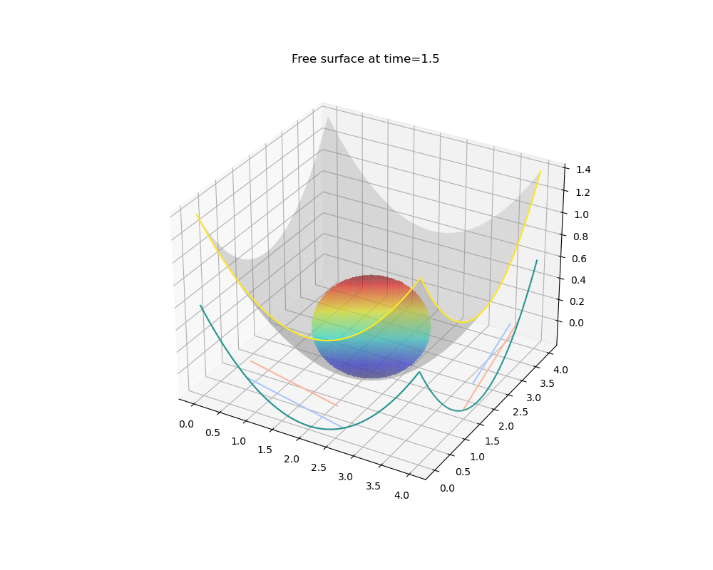
when = [0., 0.5, 1., 1.5]

thacker2d_analytic = fk.Thacker2D(triangular_mesh,
                                  a=1.,
                                  h0=0.1,
                                  compute_error=True,
                                  error_type='L2',
                                  error_output='none')

Warning

When comparisons with analytic solution have to be performed, make sure topography given to problem.layer is inherited from ‘analytic_sol’.topography

Compute analytic solution:¶

Then you can call the thacker2d_analytic() method in order to compute the analytic solution at a given time:

for time in when:
    thacker2d_analytic(time)
    create_figure(time)

plt.show()

/builds/builds/y49yFuNK/0/freshkiss3d/freshkiss3d/examples/tutorials/example_analyticsol.py:49: UserWarning: The following kwargs were not used by contour: 'color'
  csetb = ax.tricontour(triang2, scale*z, 1, zdir='x', offset=4, color='grey')
/builds/builds/y49yFuNK/0/freshkiss3d/freshkiss3d/examples/tutorials/example_analyticsol.py:50: UserWarning: The following kwargs were not used by contour: 'color'
  csetb = ax.tricontour(triang2, scale*z, 1, zdir='y', offset=0, color='grey')

Note

When solving a problem (i.e. using problem.solve()), you can pass ‘thacker2d_analytic’ trough ‘analitic_sol’ parameter that will automaticly compute analytical solution during iteration process. See API for more information.