Initialization

Simple 2-layers case with initialization examples for topography, primitives and tracer.

import numpy as np
import matplotlib.pylab as plt
import freshkiss3d as fk

functions used to plot examples:

def PLOT_VELOCITY_TOP(triangular_mesh, primitives):
    x = np.asarray(triangular_mesh.triangulation.x)
    y = np.asarray(triangular_mesh.triangulation.y)
    trivtx = np.asarray(triangular_mesh.triangulation.trivtx)
    plt.rcParams["figure.figsize"] = [10, 4]
    fig = plt.figure()
    #Subplot 1
    ax1 = fig.add_subplot(121)
    ax1.triplot(x, y, trivtx, color='k', lw=0.5)
    im1 = ax1.tricontourf(x, y, trivtx, primitives.U[:, 1], 30, cmap=plt.cm.jet)
    fig.colorbar(im1, ax=ax1)
    ax1.set_title("Velocity x component on layer {}".format(1))
    #Subplot 2
    ax2 = fig.add_subplot(122)
    ax2.triplot(x, y, trivtx, color='k', lw=0.5)
    im2 = ax2.tricontourf(x, y, trivtx, primitives.V[:, 1], 30, cmap=plt.cm.jet)
    fig.colorbar(im2, ax=ax2)
    ax2.set_title("Velocity y component on layer {}".format(1))
    plt.show()

def PLOT_U_LAYERS(triangular_mesh, primitives):
    x = np.asarray(triangular_mesh.triangulation.x)
    y = np.asarray(triangular_mesh.triangulation.y)
    trivtx = np.asarray(triangular_mesh.triangulation.trivtx)
    plt.rcParams["figure.figsize"] = [10, 8]
    fig = plt.figure()
    #Subplot 1
    ax1 = fig.add_subplot(221)
    ax1.triplot(x, y, trivtx, color='k', lw=0.5)
    im1 = ax1.tricontourf(x, y, trivtx, primitives.U[:, 0], 30, cmap=plt.cm.jet)
    fig.colorbar(im1, ax=ax1)
    ax1.set_title("Velocity x component on bottom layer")
    #Subplot 2
    ax2 = fig.add_subplot(222)
    ax2.triplot(x, y, trivtx, color='k', lw=0.5)
    im2 = ax2.tricontourf(x, y, trivtx, primitives.U[:, 1], 30, cmap=plt.cm.jet)
    fig.colorbar(im2, ax=ax2)
    ax2.set_title("Velocity x component on top layer")
    #Subplot 3
    ax3 = fig.add_subplot(223)
    ax3.triplot(x, y, trivtx, color='k', lw=0.5)
    im3 = ax3.tricontourf(x, y, trivtx, primitives.V[:, 0], 30, cmap=plt.cm.jet)
    fig.colorbar(im3, ax=ax3)
    ax3.set_title("Velocity y component on bottom layer")
    #Subplot 2
    ax4 = fig.add_subplot(224)
    ax4.triplot(x, y, trivtx, color='k', lw=0.5)
    im4 = ax4.tricontourf(x, y, trivtx, primitives.V[:, 1], 30, cmap=plt.cm.jet)
    fig.colorbar(im4, ax=ax4)
    ax4.set_title("Velocity y component on top layer")
    plt.show()

Time loop:

The simulation ends at final_time or when time iteration reach time_iteration_max.

vtk_scheduler schedules saving of the solution in VTK file. Here 10 VTK files are set for the whole simulation time.

simutime = fk.SimuTime(final_time=0.1, time_iteration_max=1000,
                       second_order=True)

vtk_scheduler = fk.schedules(count=10)

Mesh:

triangular_mesh = fk.TriangularMesh.from_msh_file('../simulations/inputs/square.msh')

Topography:

There is several ways to define topography, given the fact that it is a table of size [NC] conaining z_b values at each nodes of the mesh. One can provide a table topography from file (np.loadtxt(str(topo_file_path))) or user defined:

topography = np.zeros(triangular_mesh.NV)

See also

We could also provide a function topography_functor that returns z_b(x,y):

def topo(x, y):
    x_0 = 5
    y_0 = 5
    topo = 0.05*(x-x_0) + 0.02*(y-y_0)**2
    return topo

Layers:

Based on toporaphy initialization, topography or topography_functor should be used as argument in layer call

NL = 2
layer = fk.Layer(NL, triangular_mesh, topography=topography)
#layer = fk.Layer(NL, triangular_mesh, topography_functor=topo)

Primitives:

There is several ways to initialize these variables:

• For H we can provide water height or free_surface

• For velocities (default=0.) we can either provide QXinit, QYinit or Uinit, Vinit.

Note

For each primitive you can either provide a constant ‘Pinit’ which will be set within the entire domain or specify a function of Pinit = f(x,y) (To call functions you need to add the suffix _funct to Pinit). If you want to set different initial values on each layer you can also provide a matrix that contains value on every node of the mesh: Pinit(NC,NL).

Since topography is flat in this example defining height or free_surface is the same. First we can set U and V to simple values:

primitives = fk.Primitive(triangular_mesh, layer,
                          free_surface=1.,
                          Uinit=0.3,
                          Vinit=0.2)

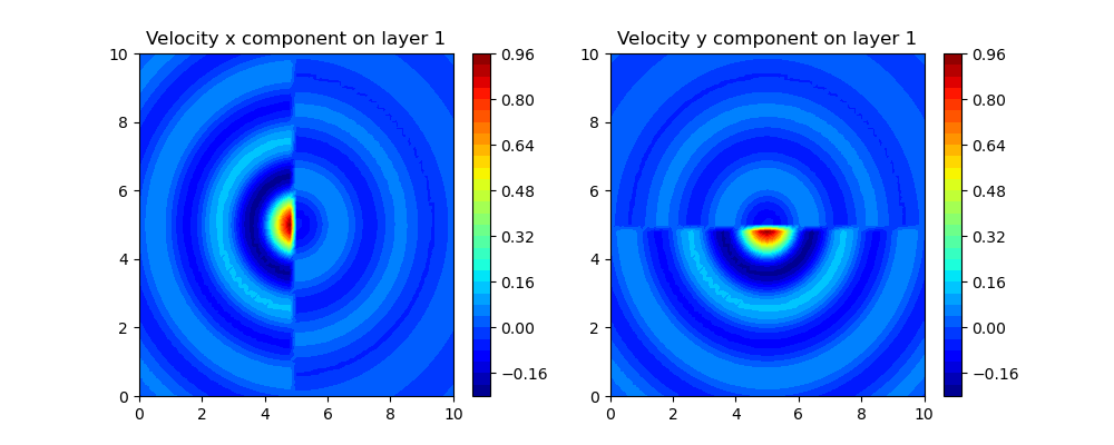
If we want to use a function to define U we can do:

def U_0(x, y):
    r = np.sqrt((x-5.0)**2+(y-5.0)**2)
    if x < 5.:
        u = np.sinc(r)
    else:
        u = np.sinc(r + np.pi)
    return u

def V_0(x, y):
    r = np.sqrt((x-5.0)**2+(y-5.0)**2)
    if y < 5.:
        v = np.sinc(r)
    else:
        v = np.sinc(r + np.pi)
    return v

primitives = fk.Primitive(triangular_mesh, layer,
                          free_surface=1,
                          Uinit_funct=U_0,
                          Vinit_funct=V_0)
#Test plot:
PLOT_VELOCITY_TOP(triangular_mesh,primitives)

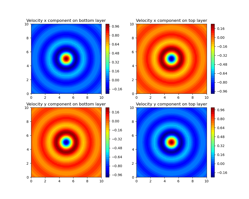
lets say we want to define specific value for each layer, we will provide the matrix Uinit(NC,NL) and Vinit(NC,NL):

NC = triangular_mesh.NV

U_0 = np.zeros((NC, NL))
V_0 = np.zeros((NC, NL))
for C in range(NC):
    x = triangular_mesh.vertices[C].x
    y = triangular_mesh.vertices[C].y
    r = np.sqrt((x-5.0)**2+(y-5.0)**2)

    U_0[C, 0] = np.sinc(r)
    U_0[C, 1] = -np.sinc(r)
    V_0[C, 0] = -np.sinc(r)
    V_0[C, 1] = np.sinc(r)

primitives = fk.Primitive(triangular_mesh, layer,
                          free_surface=1,
                          Uinit=U_0,
                          Vinit=V_0)
#Test plot:
PLOT_U_LAYERS(triangular_mesh,primitives)

See also

We have shown how to define U, V. We also could have provided QX and QY instead.

Tracer:

Like velocity there is 3 ways of defining Tinit: constant value, function (Tinit_funct) or table of size (NC,NL).

Here is an example with a simple function to define Tinit and a ‘salinity’ compressible law:

def T_0(x, y):
    if x < 5.:
        value = 30.*(x-5)**2+(y-5)**2
    else:
        value = 0.
    return value

tracer = fk.Tracer(triangular_mesh, layer, primitives, Tinit_funct=T_0)